Betwist(tm): Evolutionary Design of a Trie

I’m building Betwist(tm), a word-finding game related to Boggle®. You’re given a repeating grid of letters, and find words by moving from letter to letter.

We start with a dictionary, the set of all valid words. It’s used for two things:

Primary: When you propose a word, the system validates it.
Secondary: At the end of the game, the system tells you all the words you could have found.

Starting Point: Linear Search

To validate a proposed word, we started by loading the dictionary strings into a list and doing a linear search. With 264,000 words in the dictionary, you scan on average half the words when it’s valid, and all the words when it’s not.

Obvious Improvement: Binary Search

Since a dictionary is easily sorted, our first improvement was to do binary search. This lets you find a word (or not) in log2 time. For our dictionary, this reduces our search from thousands of attempts to at most 19.

Pretty nice for a little algorithmic tweak!

Sidebar: Required Operations

A typical search problem is “determine whether an item is in a set”. That works for testing a proposed word – “is this word in the dictionary?”

Our game has another challenge: “What are all the words in this board?”

We could just generate all possible words (following the neighboring-letter rule), but that becomes silly:

We found INORGANIC
None of its neighbors are words: INORGANICX, INORGANICA, INORGANICL
So expand INORGANICX: try INORGANICXR, INORGANICXA, INORGRANICXL
Keep expanding until you’ve attempted words up to the maximum length
That’s a lot of expanding, when the only word you could find is INORGANICALLY!

To avoid that exhausting search, we add an extra operation: “Is this the prefix of a possible word?” Then we accept INORGANIC, and only attempt to expand INORGANICA.

Both linear and binary search can accomplish this easily, using “starts with” rather than “equals”.

Trie – An Alternative Data Structure

Both linear and binary search have performance based on the size of the dictionary. There’s another parameter, though: the length of the word (or prefix).

A tried-and-true approach is the trie, an approach originally devised in 1912(!), first implemented on a computer in 1959, and named in 1960. “Trie” comes from “retrieval”, but It’s commonly pronounced “try” rather than “tree”. We already have enough trees in computer science.

A trie is a state machine built from your dictionary; the nodes indicate your progress, and the edges tell you which letters extend that prefix. Each edge has a flag telling whether it completes a word. The trie finds words in time proportional to their length.

For the words AN, BE, BED, BET, the trie looks like this:

A trie that can find "AS", "BE", "BED", and "BET".

To find a word, start at the first node and walk your word letter by letter. If you can’t find a suitable edge at any point, you don’t have a valid word or prefix. You have a word only if your last letter is marked as completing a word.

In our example, A is not a word because the “A” edge has its isWord flag false. BAT is not a word because you can only exit the second node with an “E”.

Prefix testing is straightforward: don’t check the “word complete” flag but do make sure you can take steps for each letter and could go at least one letter past your prefix. Thus A is a valid prefix, but AN, AS, and CAR are not.

Representing the State Machine

Our first version of the state machine was a direct one: nodes and pointers:

struct Trie: Codable {
  let isWord: Bool
  let next: [TrieMatch]
}

struct TrieMatch {
  let char: Character
  let trie: Trie
}

We started with the isWord flag on the Trie. (We later moved it to the TrieMatch.) Trie recursively holds an array of matches. Each match tells the character for the edge, and the subtree. We do a linear search of the array – a much smaller list than our dictionary.

The Trie approach didn’t speed up our word search significantly, but it made a noticeable difference for prefix search (over thousands of possible words in the board).

A trie is fairly expensive in terms of storage space. For our 264K words, we have about 400K nodes. I don’t have detailed statistics for the node, so I’m going to somewhat arbitrarily guess that half the nodes have an average of 4 edges, and half have 1.

A match has a character and a (pointer to a) trie. A Unicode character in Swift takes up to 7 bytes, and it’s almost certainly padded to an 8-byte boundary (64 bits) anyway. The pointer will be another 8 bytes, totaling 16 bytes per match entry.

The trie node will thus need 16 bytes for the Bool and the count, and 16 bytes per match.

So:
200K nodes * 16 bytes/node + 200K nodes * 4 matches/node * 16 bytes/match
+ 200K nodes * 16 bytes/node + 200K nodes * 1 match/node * 16 bytes/match
= 22.4 M bytes

This is about 10x as much space as our dictionary (2.7M).

Disk Space

We started by saving this structure to disk in the easiest way possible: mark the structs Codable and let Swift write them as JSON. This came out to about 4M.

JSON is a fairly redundant format: a one-line change (to compress the file before writing) reduced the file to 2.5M, which sped up the initial load but didn’t do anything about decoding time.

It took a bit less than a second to load the file – but then 5 or 6 seconds to reconstitute the structures back from the JSON.

That time left our app annoyingly slow on startup.

Complexity for Space – a Binary Trie

A sprawling data structure can often be turned into a more compact structure that’s a little harder to work with. That was our next step.

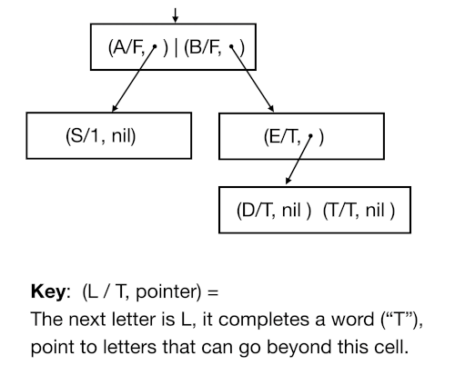
We first moved the isWord flag to the character rather than the node. Since we only care about 26 letters, we could combine the flag with a one-byte character. Our convention is that upper-case letters don’t terminate a word, while lower-case ones do.

Rather than needing an 8-byte pointer, our matches can get by with 3 bytes which can address 16M. (We only need positions up to about 4M.)

Thus, each match entry is represented by 4 bytes:
Character + isWord flag (1 byte) | offset (3 bytes)

Each trie node is just a sequence of 4-byte matches. To eliminate the implicit count of the array, we added a final node to the list marked with a 0 for its first byte.

Our original example looks like this (for AN, BE, BED, BET):

0 - 00 FF FF FF - an empty node as a boundary
1 - 41 00 00 04 - "A", 4
2 - 42 00 00 06 - "B", 6
3 - 00 FF FF FF - end of first node
4 - 6E 00 00 00 - "n", 0 - terminates "AN"
5 - 00 FF FF FF - end of node
6 - 65 00 00 08 - "e", 8 - terminates "BE" and continues
7 - 00 FF FF FF - end of node
8 - 64 00 00 00 - "d", 0 - terminates "BED"
9 - 74 00 00 00 - "t", 0 - terminates "BET"
10- 00 00 00 00 - end of node

Matches cost 4 bytes, and nodes have a one-match additional cost (for the end-of-node marker). I estimated our space needs would be noticeably smaller:

200K nodes * 5 matches/node * 4 bytes/match
+ 200K nodes * 2 matches * 4 bytes
= 5.6M

This is about 1/3 the space in RAM.

My estimate was slightly off; the real file is 4M raw, and 1.8M compressed on disk. The load time is about 1.5 seconds; much better.

Next Trie – Cutting Zeroes

In writing up all the above, I noticed that our end-of-node marker is expensive – up to 50% overhead. Of the 9 nodes in our example, 4 are markers.

In measuring the real trie, we have 586,553 regular nodes, and 417,478 marker nodes. That’s about 40% overhead.

I noticed we still have 2 bits free in our character byte. So we used one of those bits to mark the last match in a list as the end of list (eliminating the end-of-list marker).

This resulted in our trie going from 4M down to 2.3M in RAM, compressed to 1.8M on disk. It takes 1-2 seconds to load.

Squeezing Further: 3-Byte Matchers

Squeezing further cuts both time and space. Can we lower our 4-byte matchers to 3-byte ones? Yes!

We measured – the largest jump value in our state machine was 3,999,632 out of a trie size of 4,016,128. But two bytes can only represent 64K (maybe 128K if we steal that last unused bit in the character).

That number, however, was the byte offset rather than the row number. We divided those jump values by 4 (since we had 4-byte matchers). That left our biggest jump being 999,908 (about 2^20). That’s still too big for 16 bits.

Why was the biggest jump so big? It was going from the Z for the first letter to the second letter of a word that started with Z. Since we generate the trie depth-first, we do the first letter, then all the words starting with A, then the ones B, etc.

We could rework the generator to see if depth-first would make it ok, but first we did a different analysis: after the 26 first-letter matchers, what was the largest jump? It was only 63,876 (for S) – comfortably under the 65,536 limit for 16 bits.

Going to 3 Bytes

So, we reworked the meaning of the offsets again. The first 26 needed 20 bits or more, so we gave them 3-byte entries that don’t have a character value (since we know that slot[n-1] contains the nth offset). Then we defined the other offsets to be 2-byte offsets, starting from where the first-letter offset sent them.

That looks like this:

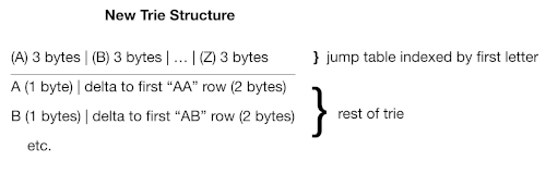
The first 26 entries are 3-byte addresses. The remaining entries are one byte for the character and 2 bytes for the row offsets.

Our final form, with 3-byte entries, takes 1.76M in RAM, and compresses to 1.4M on disk. As a bonus, it runs faster. I didn’t do enough measurement to know for sure, but I suspect that the quick lookup on the first character is what makes most of the difference (an array index, instead of a scan).

Could we get down to 2-byte matches? Perhaps, but I’ll let someone else do that investigation:)

Conclusion: Evolutionary Refinement

Our needs evolved from “Is this a word?” to also asking “Is this the proper prefix of a word?”

Our data structure evolved too, maintaining the same abstract interface:

Array with linear search (too slow)
Array with binary search (better but still slow)
Trie with direct representation (quick to use but slow to load)
Trie with “squeezed” representation (faster to load)
Trie with markers removed (notably less space)
Trie with 3-byte matchers (less space again, somewhat faster)

What made this possible?

A strong abstraction (search, search for a prefix).
A stable of candidate data structures and algorithms, with tradeoffs. (See the article on set-based concurrent engineering for more examples.)
A handful of optimization techniques.

This let us deliver a working solution early, followed by improvements on various dimensions.